Time Series Forecasting with Deep Learning: A Practical Guide

Time series forecasting is a cornerstone of data-driven decision making in finance, retail, and supply chain management. Traditional methods like ARIMA and exponential smoothing have been widely used, but deep learning has opened new possibilities for capturing complex temporal patterns. In this post, I’ll explain how to apply deep learning methods such as LSTMs, GRUs, and Transformers to time series forecasting, with practical code snippets and best practices.

Why deep learning for time series?

Classical models work well for short, stationary time series. But real-world data often includes multiple variables, non-linear relationships, and long-term dependencies. Deep learning excels here because:

• It captures non-linear relationships automatically.
• It can handle multivariate inputs (e.g., sales, weather, promotions).
• It models long-range dependencies better than ARIMA-like models.

LSTM and GRU networks

Recurrent neural networks were designed for sequential data, but suffer from vanishing gradients. LSTMs and GRUs solve this by adding gating mechanisms to retain long-term dependencies.

Example: Forecasting stock prices with LSTM

import numpy as np
import pandas as pd
import tensorflow as tf
from tensorflow.keras.models import Sequential
from tensorflow.keras.layers import LSTM, Dense

# Prepare data
X_train, y_train = create_sequences(stock_data, window_size=30)

# Define model
model = Sequential([
    LSTM(64, return_sequences=True, input_shape=(30, X_train.shape[2])),
    LSTM(32),
    Dense(1)
])

model.compile(optimizer='adam', loss='mse')
model.fit(X_train, y_train, epochs=20, batch_size=32)

The network learns temporal dependencies over 30-day windows to predict the next value.

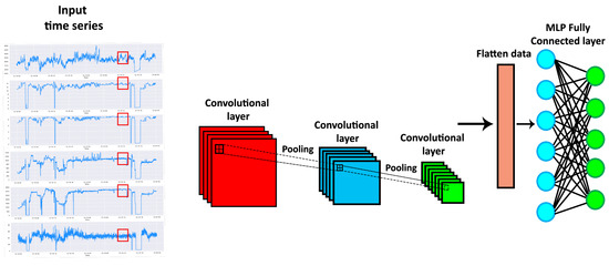
1D Convolutional models

Convolutional neural networks (CNNs) can also be effective for time series. They extract local temporal features using sliding kernels, often with faster training times than LSTMs.

Transformers for time series

Recently, transformers have been adapted for forecasting. Instead of recurrence, they use attention to model dependencies across the sequence.

Code snippet: Transformer block

from tensorflow.keras.layers import MultiHeadAttention, LayerNormalization, Dropout, Dense

class TransformerBlock(tf.keras.layers.Layer):
    def __init__(self, embed_dim, num_heads, ff_dim, rate=0.1):
        super(TransformerBlock, self).__init__()
        self.att = MultiHeadAttention(num_heads=num_heads, key_dim=embed_dim)
        self.ffn = Sequential([
            Dense(ff_dim, activation="relu"),
            Dense(embed_dim),
        ])
        self.layernorm1 = LayerNormalization(epsilon=1e-6)
        self.layernorm2 = LayerNormalization(epsilon=1e-6)
        self.dropout1 = Dropout(rate)
        self.dropout2 = Dropout(rate)

    def call(self, inputs, training):
        attn_output = self.att(inputs, inputs)
        attn_output = self.dropout1(attn_output, training=training)
        out1 = self.layernorm1(inputs + attn_output)
        ffn_output = self.ffn(out1)
        ffn_output = self.dropout2(ffn_output, training=training)
        return self.layernorm2(out1 + ffn_output)

Transformer-based models such as Informer and Temporal Fusion Transformer achieve state-of-the-art performance in forecasting tasks with long sequences.

Best practices

• Data preprocessing. Normalize inputs, handle missing values, and engineer calendar features (day of week, holiday).
• Windowing. Forecasting models require sliding windows of past observations. Experiment with window size.
• Evaluation metrics. Use MAPE, RMSE, and business-specific KPIs.
• Regularization. Dropout, early stopping, and simpler architectures prevent overfitting.

Case study: Retail demand forecasting

For a retail client, we used an LSTM-based model with external features such as holidays and promotions. The model improved forecast accuracy by 12% compared to a baseline ARIMA. Crucially, we added explainability via SHAP values to understand which external features influenced demand the most.

Common pitfalls

• Overfitting to historical data that doesn’t generalize to future trends.
• Ignoring seasonality and external drivers.
• Using too complex a model when simpler baselines perform well.

Conclusion

Deep learning has expanded the toolkit for time series forecasting. LSTMs and GRUs capture sequential dependencies, CNNs extract local patterns efficiently, and transformers enable long-range forecasting. The key is to match the model to the business problem, ensure data quality, and evaluate against strong baselines. With the right practices, deep learning can unlock significant improvements in forecasting accuracy for financial services, retail, and beyond.

"In time series forecasting, the real challenge is not just predicting the future but doing so in a way that is robust to the unexpected." – Ashish Gore

If you’d like to explore forecasting architectures for your use case, feel free to reach out via my contact information.